Reporting Formulas

Last updated
Save as PDF

This topic provides an overview to working with formulas in TeamConnect Business Intelligence along with important tips and examples.

Formulas are custom calculations performed on one or more fields in your data. They offer an important way to analyze results and express business logic. The formula capabilities are designed around several principles:

Create complex business calculations without IT or technical knowledge.
Easily combine fields from different data sources together.
Customize formulas to reflect specific criteria and conditions.
Work with raw data without the need to summarize data sets before creating formulas.
Instantly recalculate formulas based on any filter, variable or level of granularity.

Use the Formula Editor to create formulas that define the values and filters of a widget.

The following table provides a reference to the main formula functions.

Goal	Function	Types and Syntax
Perform calculation based on criteria	Measured value	Value Filters: ≠ , =, >, <, between Text Filters: Contains, Doesn't Contain, Doesn't End With, Doesn't Start With, Ends With, Start With, Equals, Not Equal List Filter: Include, Exclude Ranking Filters: Top, Bottom Ranking Time Filter: Date and Calendar
Combine data/apply simple mathematics	Aggregate functions	Operator: +,-,,/ Aggregate: Sum() Average: Avg() Count: Count(), DupCount() Range*: Max()/Min()
Summarize data	Statistical function	Central Tendency: Median(), Model, Largest() Std Deviation and Variance: Stdev(), Stdevp(), Varp(), Var() Quartile and Percentile: Quartile(), Percentile()
Accumulate data	Rolling sum/average	Sum to Date: YTDSum(), QTDSum, MTDSum() Avg to Date: YTDAvg, QTDAvg, MTDAvg()
Compare Time or Trends	Time functions	Past Periods: PastYear(), PastQuarter(), PastMonth(), Next(), Prev() Growth Trend: Growth(), GrowthRate() Time Difference: YDiff(), QDiff(), MDiff(), DDiff(), HDiff(), MnDiff(), SDiff()

Using the Formula Editor

The Formula Editor is where Designers define formulas for a dashboard widget.

To open the Formula Editor:

For a new widget, click Select Data, and then the function button.
For an existing widget, click the edit formula button.

The Formula Editor consists of two tabs, the Data Navigator to select fields, and the Functions tab to select formula operations. It is possible to create a combination of one or more functions, fields and filters. The following diagram outlines the major components of the formula.

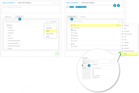
Functions are operations which carry out various calculations, for example a sum. Use the Jump To menu or the search box to quickly find the formula you need.
Fields in the Data Browser are variables contained in the data set (ElastiCube). Clicking a field in the data browser will include it as part of the formula.
Filters can be applied to restrict formulas based on criteria.
Starring is a way to save a formula as a favorite for later use.
The Formula Editor window can be expanded by clicking the expand button at the top right.

Creating and Editing a Formula for a Widget

The Data Browser enables you to define formulas (freeform expressions) that define the values and filters of a widget.

To define a formula:

Click on the Formula Editor in the Data Browser. The Data Browser will display the Formula Editor on the screen, which has two tabs:
- The Data Browser tab provides fields to choose from.
- The Functions tab lists the functions that you can include in your formula by selecting them. You can read a description of each function in a tooltip by hovering over it.
Define the formula as follows:
- From the Data Browser tab, select one or more fields.
- From the Functions tab, select the required functions.
The formula's required elements must be typed in. For examples, see Formulas Based on Criteria and Conditions, and Functions to Build Formulas.
Click OK.

To edit a formula, right-click on the formula and select one of the following from the context menu:

Rename: Rename the formula, for example, give a name that represents a real-life task (or) expected result from the formula, (or) include in the name filters that you have added to the formula.
Filter: Add filters to the formula.
Type: Change the default aggregation method, for example, from Sum to Average.

Reusing Formulas

Users can reuse formulas that they have marked as a favorite (starred).

Note: A starred formula can be changed, but earlier applications will continue to utilize the previous version of the formula. Only future applications of the starred formula will utilize your latest formula.
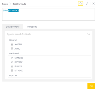
To mark a formula as a Favorite:

While defining a formula, click on Favorite (Star) button.
Enter a name for the formula.
Click on OK.

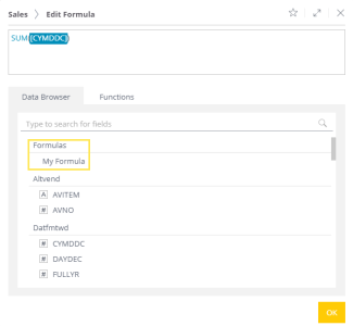
To reuse a favorite formula, select it from the Data Browser tab.

Using Quick Functions

Quick functions are the another feature to make working with formulas easier similar to reusing formulas. When selecting a value to be included in a widget, the Widget Designer provides a number of predefined, frequently used functions that users can quickly apply in the Data Browser.

Quick Functions instantly add a time dimension to any existing value and formula. These functions include calculations for past values, change over time, contribution and running totals. Quick Functions include all the Time Functions previously discussed, but they can only be accessed by clicking a formula that is already present in a widget.

To use a quick function:

Click on the menu icon of a numeric field in the data panel of the widget designer and then select Quick Functions from the menu. A list of commonly used functions will be displayed.
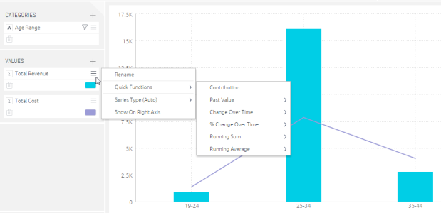
Select a function. The widget will be updated immediately.

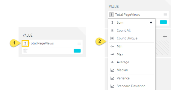
To add aggregate functions to your formula without opening the formula editor, click on Value icon and select the function to apply to your formula.

Creating Formulas Based on Criteria and Conditions (Filters)

Often formulas must take into account specific criteria. Measured Value is a feature that, similar to the SUMIF function in Excel, only does calculations when the values meet a set of criteria. Criteria for Measured Values can be based on any logical operators in a filter.

To filter the formula:

In the Data Browser, create the formula from the Data Browser and Functions tabs, as explained in Formula Editor.
Add the field (or criteria) by which you want to filter the formula. Right-click on the field and select Filter.
Users can then filter the formula by listed items, text options, ranking, etc. When done, click on OK.

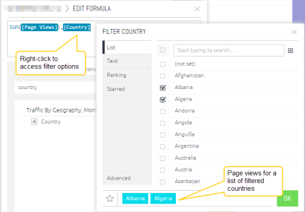
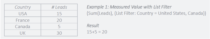
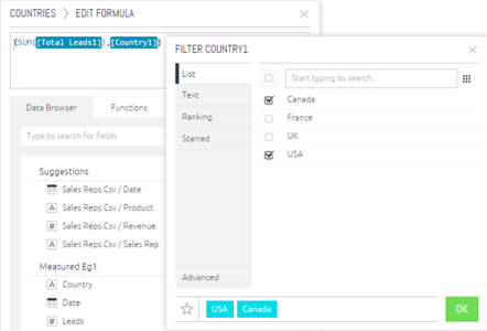
Below the simple example of Measured Value which is the use of a list filter. A marketing team may need to count leads generated for a specific region such as North America. Even if leads come from many different countries, the measured value calculates leads generated only when the lead originates from the United States or Canada.

In the Formula Editor, the scenario described above can be defined as follows:

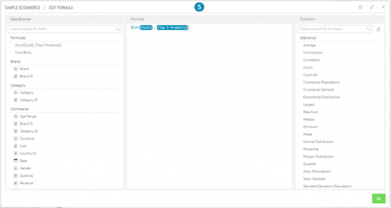
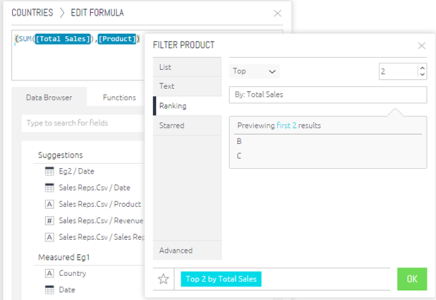
Use of a ranking filter is an example of more complicated scenario. For example a sales team may want to track the contribution of best-selling products to total revenue. However, what constitutes a popular product may change over time. A measured value can be created for sales, which includes a condition that only shows sales of the top products for any month. This simultaneously filter the data, but also takes into account changes in what classifies as a top product over time.

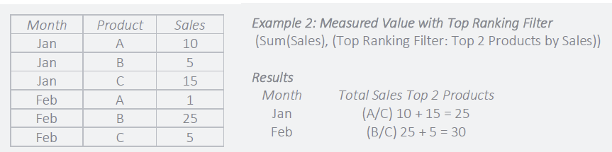
In the Formula Editor, the scenario described above can be defined as follows:

Measured Values are a powerful feature to take into account business logic and quickly perform calculations only when a specific set of criteria is met.

Note: If your widget is filtered using measured values, then the measured value will override any other widget or dashboard filters you have for the same fields.

Creating Conditional Color-coded Charts

Users can able to create conditional formulas that reflect as color-coded charts within widgets. This creates a quick, easy way to visually identify trends. Follow the instructions below to set up conditional colors.

Note:

This process should be completed by a system administrator who has designer rights.
Conditional states work on measures and aggregations only and return numeric values.

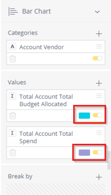
Navigate to the Reports tab and select the visualization report (any report widget). Find the functions on the left sidebar that indicates where colors can be changed.
Click one of the colors and select the Conditional Tab. Here, users will set up the conditions for color indicators. Users can create intervals using multiple conditions.
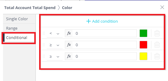
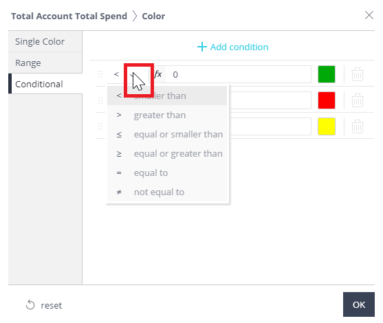
Click on the Dropdown (down arrow) to set the operator and colors.

Each condition must have an operator (greater than, less than, equal to), an interval (shown in step 4), and a color selection. In this example, the operator is comparing itself to the Total Account Total Spend. So everything listed after the operator will be compared to Total Account Total Spend.

Note: The system evaluates the conditions chronologically, so set them up accordingly.
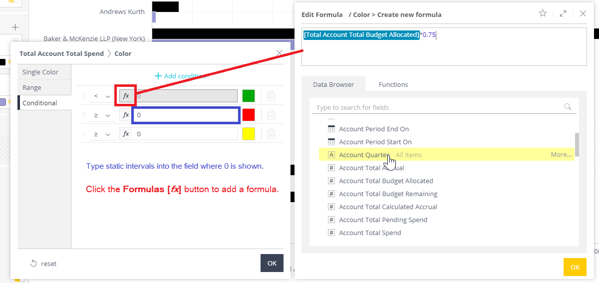
Set the intervals and colors. Intervals can reference static amounts, or calculations using formulas (select the fx icon). Formulas can be combinations of rational numbers, functions, and field data.

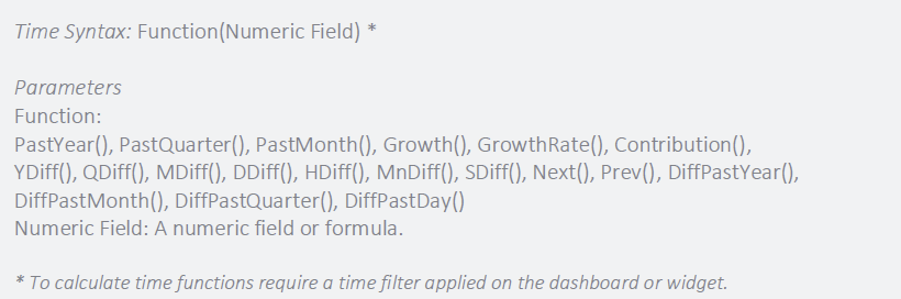
If using a function, there is a list of available options to browse. When the user hovers over a specific function, the syntax that must be followed for the function is included in a popup window.
Click Ok, when completed.
Repeat this process as necessary to get your desired conditions and colour choices.

Note: In the widget, the total Account Total Spend shows as a grey color in the chart's legend at the bottom of the table. This is beacse the table doesn't separate out the conditional colors so it appears as grey.

Building Formulas with Functions

Functions are operations that perform common types of calculations, and can be used to build formulas. This section describes four types of functions.

Combine Data: Aggregate Functions

To do mathematical computations on data, aggregations are used. To quickly summarize data based on multiple factors, users can execute multiple aggregations on several fields concurrently.

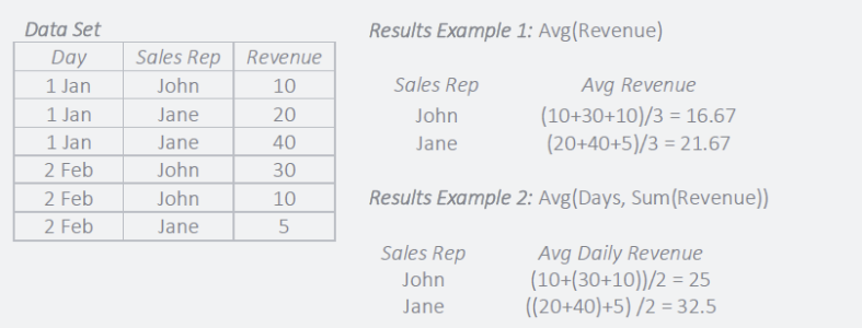
For example, a sales manager can create a pivot table to show the average sales revenue for each sales representative.

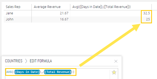
A more complex example is a multi-pass aggregation (or grouping) that is an aggregation that performs multiple calculations simultaneously. The sales manager wants to also see average sales per day for each sales representative. Instead of having to add an additional column for a day in the pivot table, the manager can create a multi-pass aggregation that first performs a sum of sales per day and then averages the results for each rep. This requires two fields – a day from a date field and the revenue field, as well as two aggregations, sum of sales and average. The result is the sales manager does not need to add a column for days in the pivot.

Summarize Data: Statistical Functions

In especially for big data sets where descriptive statistics can help to focus investigation, descriptive statistics give relevant summaries of data and aid in making better informed judgements.

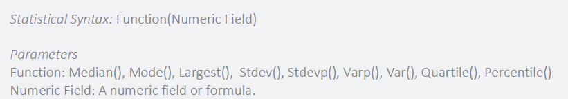
An example of statistical functions is a marketing team that has a large data set of leads generated from various channels and want to understand where to focus their budget. Descriptive statistics can be used to summarize valuable insight about each channel such as the central tendency or median leads generated along with standard deviations to assess typical lead volume.

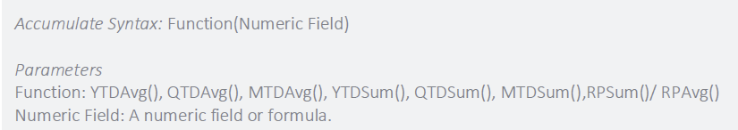
Accumulate Data: Running Total and Average

Often, data must be seen in a continuous and cumulative trend across lengthy periods, such as years, quarters, or months, in order to measure performance. Running totals and averages over predetermined or customised time periods can be created using functions.

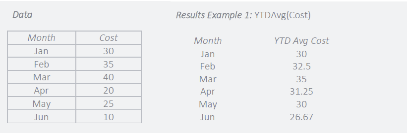
For example, a support team has a goal to reduce the average monthly cost to resolve open issues. A Year to Date Average can be used to track progress towards reducing the average cost of support.

Change over Time: Time Functions

Business decisions depend heavily on time, and Time Functions make it simple to compare outcomes over intervals of time, estimate growth rates, and compute time differences. Functions can be configured for both custom and common time periods, such as year, month, or day.

For example, an executive team wants to compare growth in revenue to the same period in the previous year. A difference in Past Year function can be used to compare past values based on the current month to the same month in the previous year.

Function Reference

The following tables list of the functions you can use in the formula editor:

Statistical Functions
Mathematical Functions
Time-Related Functions
Other Functions

Statistical Functions

Name	Function	Description	Example
Average	Avg(<numeric Field>)	Calculates the mean average of the given values	Avg(Score) will calculate the mean average of the given scores. Avg(<group by field>, <aggregation>) calculates the average of the given aggregation grouped by another filed. Avg( Product, Total Sales) will calculates the average of the total sales per product.
Contribution	Contribution(<numeric field>)	Calculates the percentage of total.	Contribution( Total Sales ) calculates the percentage of total sales per group (for example per day or per product) out of total sales (for all days or all products).
Correlation	CORREL(<Numeric Field a>, <Numeric Field b>)	Returns the correlation coefficient of two numeric fields.	CORREL(Revenue, Cost) will return the correlation between revenue and cost. CORREL(<group by field>, <aggregation a>, <aggregation b>)returns the correlation coefficient of two fields aggregations grouped by another field. CORREL(Products, AVG(Revenue), AVG(Cost)) will return the correlation between the average of revenue and cost per product.
Count	Count(<Numeric Field>)	Counts the number of unique values within the given values.
Count All	DupCount(<Numeric Field>)	Returns the actual item count of the given list of items, including duplicates.
Covariance (Population)	COVARP(<Numeric Field a>, <Numeric Field b>)	Returns the population covariance of <Numeric Field a> and <Numeric Field b>.	COVARP(Revenue, Cost) will return the population covariance of revenue and cost. COVARP(<group by field>, <aggregation a>, <aggregation b>) returns the population covariance of two fields aggregations grouped by another field. COVARP(Products, AVG(Revenue), AVG(Cost)) will return the population covariance of the average revenue and the average cost per product.
Covariance (Sample)	COVAR(<Numeric Field a>, <Numeric Field b>)	Returns the sample covariance of <Numeric Field a> and <Numeric Field b>.	COVAR(Revenue, Cost) will return the sample covariance of revenue and cost. COVAR(<group by field>, <aggregation a>, <aggregation b>) Returns the sample covariance of two fields aggregations grouped by another field. COVAR(Products, AVG(Revenue), AVG(Cost)) will return the sample covariance of the average revenue and the average cost per product.
Exponential Distribution	EXPONDIST(<numeric value>, <lambda>, <Cumulative (true/false)>)	Returns the exponential distribution for a given value and a supplied distribution parameter lambda. Cumulative: TRUE = Cumulative distribution function, FALSE = Probability density function. EXPONDIST( Count(Leads), 2, False ) will return the exponential distribution density of the number of leads per country where lambda is 2.
Intercept	INTERCEPT(<field>, <numeric value>)	Returns the intercept of the linear regression line through a supplied series of x- and y- values.	INTERCEPT(Date.Quarter, Total Sales) will return the intercept of the regression line that represents the trend over quarter of the sum of sales. Largest LARGEST(<Numeric Field>, <k>) returns the k-th largest value in a field.
Maximum	Max(<Numeric Field>)	Returns the maximum value among the given values.
Median	MEDIAN( <Numeric Field> )	Calculates the median of the given values. The median of a set of data is the middlemost number in the set. The median is also the number that is halfway into the set.
Minimum	Min(<Numeric Field>)	Returns the minimum value among the given values.
Mode	MODE(<Numeric Field>)	Returns the most frequently occurring value from the column.
Normal Distribution	NORMDIST(<Numeric Field>, <Mean>, <Standard Deviation>, <Cumulative (true/false)>)	Returns the standard normal distribution for a given value, a supplied distribution mean and standard deviation. Cumulative: TRUE = Cumulative Normal Distribution Function, FALSE = Normal Probability Density Function.	NORMDIST(Score, ( Mean(Score), All(Score)), ( STDEV(Score), All(Score) ), False ) will return the normal probability density of a given score.
Percentile	PERCENTILE(<Numeric Field>, <k>)	Returns the k-th percentile value from the given field. k is any number between 0..1 (inclusive).
Possion Distribution	POISSONDIST( <numeric value>, <mean>, <Cumulative (true/false)>)	Returns the poisson distribution for a given value and a supplied distribution mean. Cumulative: TRUE = Cumulative distribution function, FALSE = Probability mass function.	POISSONDIST( Score, ( Mean(Score), All(Score) ), ( STDEV(Score), All(Score) ), False ) will return the poisson probability density of a given number of sales
Quartile	QUARTILE(<Numeric Field>, <k>)	Returns the k-th quartile for the given field. k = 0 returns the Minimum value k = 1 returns the first quartile (25th percentile) k = 2 returns the Median value (50th percentile) k = 3 returns the third quartile (75th percentile) k = 4 returns the Maximum value
Rank	RANK(<numeric value>, [DESC/ASC], [Rank Type], [<group by field 1>,... , <group by field n>])	Returns the rank of a value in a list of values [DESC/ASC] – Optional. By default sort order is descending. [Rank Type] – Optional. By default the type is standard competition ranking (“1224” ranking). Support also modified competition ranking (“1334” ranking), dense ranking (“1223” ranking) and ordinal ranking (“1234” ranking). [<Group by field 1>,… , <Group by field n>] – Optional. Rank partitions fields.	RANK(Total Cost, “ASC”, “1224”, Product, Years) will return the rank of the total annual cost per each product were sorted in ascending order.
Running Sum (RSUM)	RSUM ( <numeric value> ), RSUM ( <numeric value> , <continuous> )	Returns the running total of the measure by the defined dimension according to the current sorting order in the widget. By default, RSUM accumulates a measure by the sorting order of the dimension. To accumulate by another order, the relevant measure should be added as an additional column and sorted. <continuous> is a boolean value that that accumulates the sum continuously when there are two or more dimensions. The default value is False. Note: Filtering the RSUM column by Values, filters the dimensions and recalculates the RSUM from the first filtered value.
Skewness (Population)	SKEWP(<numeric value>)	Returns the skewness of the distribution of a given value in the population.	SKEWP(Revenue) will return the skewness of the distribution of revenue in the population.
Skewness (Sample)	SKEW(<numeric value>)	Returns the skewness of the distribution of a given value.	SKEW(Revenue) will return the skewness of the distribution of revenue.
Slope	SLOPE(<field>, <numeric value>)	Returns the slope of the linear regression line through a supplied series of x- and y- values.	SLOPE(Date.Quarter, Total Sales) will return the slope of the regression line that represent the trend over quarter of the sum of sales.
Standard Deviation (Population)	STDEVP( <Numeric Value> )	Returns the Standard Deviation of the given values (Population). Standard deviation is the square root of the average squared deviation from the mean. The standard deviation of a population gives researchers the amount of dispersion of data for an entire population of survey respondents.
Standard Deviation (Sample)	STDEV( <Numeric Value> )	Returns the Standard Deviation of the given values (Sample). Standard deviation is the square root of the average squared deviation from the mean. A standard deviation of a sample estimates the amount of dispersion in a given data set, based on a random sample.
T Distribution	TDIST( <numeric value x>,<degrees_freedom>, <Cumulative (true/false)>)	Returns the student’s T-distribution for a given value and a supplied number of degrees of freedom (must be ≥ 1). Cumulative: TRUE = Cumulative Distribution Function, FALSE = Probability Density Function.	TDIST( Score, 3, TRUE ) will return the student’s T-distribution of a given score, with 3 degrees of freedom.
Variance (Population)	VARP( <Numeric Value> )	Returns the Variance of the given values (Population). Variance (Sample) is the average squared deviation from the mean, based on an entire population of survey respondents.
Variance (Sample)	VAR( <Numeric Value> )	Returns the Variance of the given values (Sample). Variance (Sample) is the average squared deviation from the mean, based on a random sample of the population.

Mathematical Functions

Name	Function	Description	Example
Absolute	Abs(<Numeric value>)	Returns the absolute value of the given value.	ABS(Cost), where the absolute result for the value ‘2’ or ‘-2’ is ‘2’.
Acos	ACOS(<numeric value>)	Returns the angle, in radians, whose cosine is the given numeric expression. Also referred to as arccosine.	ACOS(Total Revenue) will return the angle, in radians, whose cosine is the given total revenue.
Asin	ASIN(<numeric value>)	Returns the angle, in radians, whose sine is the given numeric expression. Also referred to as arcsine.	ASIN(Total Revenue) will return the angle, in radians, whose sine is the given total revenue.
Atan	ATAN(<numeric value>)	Returns the angle in radians whose tangent is the given numeric expression. Also referred to as arctangent.	ATAN(Total Revenue) will return the angle in radians whose tangent is the given total revenue.
Ceiling	CEILING(<numeric value>)	Returns number rounded up, away from zero, to the nearest multiple of significance.	CEILING(Cost), where the result of ‘83.2’ rounded up is ’84’.
Cos	COS(<numeric value>)	Returns the trigonometric cosine of the given angle (in radians).	COS(Average Angle) will return the trigonometric cosine of the average angle.
Cosh	COSH(<numeric value>)	Returns the hyperbolic cosine of the given value.	COSH(Total Revenue) will return the hyperbolic cosine of the total revenue.
Cot	COT(<numeric value>)	Returns the trigonometric cotangent of the given angle (in radians).	COT(Average Angle) will return the trigonometric cotangent of the average angle.
Exp	EXP(<numeric value>)	Returns the exponential value of the given value.	EXP(Sales) will return the exponential value of sales.
Floor	FLOOR(<numeric value>)	Returns number rounded down, toward zero, to the nearest multiple of ‘1’.	FLOOR(Revenue), where the result of ‘88.6’ rounded down is ’88’.
Ln	LN(<numeric value>)	Returns the base-e logarithm of the given value.	LN(Cost) will return the base-e logarithm of cost.
Log10	LOG10(<numeric value>)	Returns the base-10 logarithm of the given value.	LOG10(Revenue) will return the base-10 logarithm of revenue.
Mod	MOD(<numeric value>, divisor)	Returns the remainder after a number is divided by a divisor.	MOD(Cost, 10), where the reminder of ‘255’ divided by ’10’ is ‘5’.
Power	Power(value, power)	Returns the results of the given value raised to a supplied power.	POWER(Revenue, 2) will return revenue raised by the power of 2.
Quotient	QUOTIENT(<numeric value>, divisor)	Returns the integer portion of a division.	QUOTIENT(Cost, 2), where the integer portion of ‘5’ divided by ‘2’ is ‘2’.
Round	ROUND(<numeric value>, num_digits)	Returns number rounded to a specified number of digits.	ROUND(Revenue, 2) will return the revenue rounded to two decimal places.
Sin	SIN(<numeric value>)	Returns the trigonometric sine of the given angle (in radians).	SIN(Average Angle) will return the trigonometric sine of the average angle.
Sinh	SINH(<numeric value>)	Returns the hyperbolic sine of the given value.	SINH(Total Revenue) will return the hyperbolic sine of the total revenue.
Square root	SQRT(<Numeric value>)	Returns the square root of the given value.	SQRT(Cost) will return the square root of cost.
Sum	Sum(<Numeric Field>)	Calculates the total of the given values.
Tan	TAN(<numeric value>)	Returns the trigonometric tangent of the given angle (in radians).	TAN(Average Angle) will return the trigonometric tangent of the average angle.
Tanh	TANH(<numeric value>)	Returns the hyperbolic tangent of the given value.	TANH(Total Revenue) will return the hyperbolic tangent of the total revenue.

Time Related Functions

Name	Function	Description	Example
Day Difference	DDiff( <Start Time>, <End Time> )	Returns the difference between <Start Time> and <End Time> in days.
Growth	Growth( <Numeric Value> )	Calculates growth over time. The time dimension to be used is determined by the time resolution in the widget/dashboard. Formula: (current value – compared value) / compared value.	If this month your value is 12, and last month it was 10, your Growth for this month is 20% (0.2). Calculation: (12 – 10) / 10 = 0.2 If this year your value is 80, and last year it was 100, your Growth for this year is -20% ( -0.2). Calculation: (80 – 100) / 100 = -0.2
Hour Difference	HDiff( <Start Time>, <End Time> )	Returns the difference between <Start Time> and <End Time> in hours.
Prev	Prev( <Time Field> [, <N>] )	Returns the Time period Member in <Time Field> which is N periods back from the current Member. This function only works as a scope function and not by itself.	This formula will return the numeric value 2 months ago: (<Numeric Value>, Prev(<Month Field>, 2))
Minute Difference	MnDiff( <Start Time>, <End Time> )	Returns the difference between <Start Time> and <End Time> in minutes.
Month Difference	MDiff( <Start Time>, <End Time> )	Returns the difference between <Start Time> and <End Time> in months. Returns whole numbers.
Month to Date Average	MTDAvg( <Numeric Value> )	Returns the running average starting from the beginning of the month up to the current time period member.The time dimension to be used is determined by the time resolution in the widget/dashboard. Returns 0 if the active time resolution is quarters or years.
Month to Date Sum	MTDSum( <Numeric Value> )	Returns the running total starting from the beginning of the month up to the current time period member. The time dimension to be used is determined by the time resolution in the widget/dashboard. Returns 0 if the active time resolution is quarters or years.
Next	Next( <Time Field> [, <N>] )	Returns the Time period Member in <Time Field> which is N periods after the current Member. This function only works as a scope function and not by itself.	This formula will return the numeric value 2 months ahead of now: (<Numeric Value>, Next(<Month Field>, 2)
Now	Now(<Day from Date field>)	Returns the value for the current time period. Supports day, month, quarter or year. The Now function receives a date dimension and its level and returns all the members in that dimension which match the current query execution time. Note: This function only works as a scope function and not by itself.	The following example will return the value for the current day.( [Total Sales], Now([Days in Datefield]))
Past Year	PastYear( <Numeric Value> )	Calculates the value for the same period in the past (previous) year.	If you’re looking at a specific day, you will see the value of the same day one year back. If you’re looking at a specific month, you will see the value of the same month one year back. Note: When using the Past Year function in a weeks table and using a week filter, no results are returned.
Past Quarter	PastQuarter( <Numeric Value> )	Calculates the value for the same period in the past (previous) quarter.	If you’re looking at a specific day, you will see the value of the same day one quarter back. If you’re looking at a specific month, you will see the value of the same month one quarter back.
Past Month	PastMonth( <Numeric Value> )	Calculates the value for the same period in the past (previous) month.	If you’re looking at a specific day, you will see the value of the same day one month back.
Quarter Difference	QDiff( <Start Time>, <End Time> )	Returns the difference between <Start Time> and <End Time> in quarters. Returns whole numbers.
Quarter to Date Average	QTDAvg( <Numeric Value> )	Returns the running average starting from the beginning of the quarter up to the current time period member. he time dimension to be used is determined by the time resolution in the widget/dashboard, Returns 0 if the active time resolution is years.
Quarter to Date Sum	QTDSum( <Numeric Value> )	Returns the running total starting from the beginning of the quarter up to the current time period member. The time dimension to be used is determined by the time resolution in the widget/dashboard. Returns 0 if the active time resolution is years.
Range	range( <Field1>, <Field2> )	Returns a graphical range selector for a data set where two members of the same dimension and level define the minimum and maximum values of the range.
Second Difference	SDiff( <Start Time>, <End Time> )	Returns the difference between <Start Time> and <End Time> in seconds.
Year Difference	YDiff( <Start Time>, <End Time> )	Returns the difference between <Start Time> and <End Time> in years. Returns whole numbers.
Year to Date Average	YTDAvg( <Numeric Value> )	Returns the running average starting from the beginning of the year up to the current time period member. The time dimension to be used is determined by the time resolution in the widget/dashboard.
Year to Date Sum	YTDSum( <Numeric Value> )	Returns the running total starting from the beginning of the year up to the current time period member.	The time dimension to be used is determined by the time resolution in the widget/dashboard.

Other Functions

Name	Function	Description	Example
All	All(<Field>)	Ignores the scope set on the dimension.
Ordering	ORDERING(<expression1>,<expression2>)	Returns the numeric order position of rows sorted into ascending or descending order, breaking ties with further arguments. The expressions must be aggregated by applying the MIN/MAX functions as in the example.	ORDERING(MIN([Sales Person Name]), MIN([Days in Transaction_Date]), -1*Sum([Sales]))
Rdouble	RDOUBLE(<R expression>, <numeric value 1>, [<numeric value 2>, ..., <numeric value n>] )	Returns a numeric result for a given R expression and a list of numeric values (use ‘args’ in the R expression to reference numeric values parameters). The R expression is passed to the running Rserve.The optional ordering expression determines the order in which the rows are sent to R. The argument of the Ordering parameter can be an index in your data source or you can use the ORDERING() function to determine the order of the field.	RDOUBLE(“m <- log(matrix(unlist(args), ncol=2)); kmeans(m,3)$cluster”, [Total Cost], [Total Revenue]) will return the k-means cluster (R expression) of the args: [Total Cost] and [Total Revenue]. RDOUBLE(<recycle>, <R expression>, <numeric value 1>, [<numeric value 2>, ..., <numeric value n>] ) recycle = TRUE (default) – Results will be cached for unchanged functions and data. recycle = FALSE – Results will not be cached. Use this option if your R code contains randomality.
Rint	RINT(<R expression>, <numeric value 1>, [<numeric value 2>, ..., <numeric value n>] )	Returns an integer result for a given R expression and a list of numeric values (use ‘args’ in the R expression to reference numeric values parameters). The R expression is passed to the running Rserve. The optional ordering expression determines the order in which the rows are sent to R. The argument of the Ordering parameter can be an index in your data source or you can use the ORDERING() function to determine the order of the field.	RINT(“m <- log(matrix(unlist(args), ncol=2)); kmeans(m,3)$cluster”, [Total Cost], [Total Revenue]) will return the k-means cluster (R expression) of the args: [Total Cost] and [Total Revenue]. RINT(<recycle>, <R expression>, <numeric value 1>, [<numeric value 2>, ..., <numeric value n>] ) recycle = TRUE (default) – Results will be cached for unchanged functions and data. recycle = FALSE – Results will not be cached. Use this option if your R code contains randomality.